Is it a banger? Audio classification in tensorflow

In Parks and Recreation Season 6 Episode 18 “Prom”, Tom Haverford famously tells us about his test of whether a song is a “banger” or not. There are many questions in this test: “does it feature any acoutic instruments?”, “how many drops?”, “how dope are the drops?” etc.
I think we can make his test even more rigorous: why don’t we use a deep neural network, trained on examples of bangers (and non-bangers), to tell us if a song is banger or not?
In this jupyter notebook, we’re going to construct, train and test this neural network.
Initial Environment
import matplotlib.pyplot as plt
import librosa.display
import numpy as np
np.random.seed(1337)
import pandas as pd
%matplotlib inline
The Dataset
df = pd.read_pickle("../data/processed_dataset.pkl")
This data set was generated using the instructions in this notebook. Let’s take a look.
df[:9]
| audio | label | label_one_hot | log_specgram | |
|---|---|---|---|---|
| Cliff Richard - Greatest Hits 1958-1962 (Not Now Music) [Full Album]_0415.wav | [0.0, 0.0, 0.0, 0.0, 0.0, 0.0, 0.0, 0.0, 0.0, ... | not_a_banger | [1.0, 0.0] | [[-80.0, -54.1524, -35.3907, -33.0633, -39.626... |
| Selected New Year Mix_0121.wav | [0.0, 0.0, 0.0, 0.0, 0.0, 0.0, 0.0, 0.0, 0.0, ... | banger | [0.0, 1.0] | [[-67.3112, -51.5708, -53.4622, -72.6484, -80.... |
| Rihanna - Stay ft. Mikky Ekko_0036.wav | [0.0, 0.0, 0.0, 0.0, 0.0, 0.0, 0.0, 0.0, 0.0, ... | not_a_banger | [1.0, 0.0] | [[-64.2413, -50.564, -57.0061, -37.2135, -37.0... |
| The Lumineers - Slow It Down (Live on KEXP)_0049.wav | [0.0, 0.0, 0.0, 0.0, 0.0, 0.0, 0.0, 0.0, 0.0, ... | not_a_banger | [1.0, 0.0] | [[-80.0, -73.9336, -59.1297, -49.4456, -45.314... |
| Passenger _ Let Her Go (Official Video)_0016.wav | [0.0, 0.0, 0.0, 0.0, 0.0, 0.0, 0.0, 0.0, 0.0, ... | not_a_banger | [1.0, 0.0] | [[-80.0, -79.4122, -63.2455, -56.2228, -56.834... |
| Low Steppa - Vocal Loop (Premiere)_0032.wav | [0.0, 0.0, 0.0, 0.0, 0.0, 0.0, 0.0, 0.0, 0.0, ... | banger | [0.0, 1.0] | [[-65.6515, -31.3697, -21.9142, -25.2813, -61.... |
| Stardust - Music Sounds Better (Mistrix Dub) (Free Download)_0049.wav | [0.0, 0.0, 0.0, 0.0, 0.0, 0.0, 0.0, 0.0, 0.0, ... | banger | [0.0, 1.0] | [[-80.0, -80.0, -78.6725, -79.2538, -80.0, -80... |
| Ed Sheeran - Thinking Out Loud [Official Video]_0033.wav | [0.0, 0.0, 0.0, 0.0, 0.0, 0.0, 0.0, 0.0, 0.0, ... | not_a_banger | [1.0, 0.0] | [[-80.0, -65.3586, -53.2574, -44.407, -50.1324... |
| Best Of 2017 Tech House Yearmix_0145.wav | [0.0, 0.0, 0.0, 0.0, 0.0, 0.0, 0.0, 0.0, 0.0, ... | banger | [0.0, 1.0] | [[-80.0, -57.0543, -39.8118, -61.7071, -38.360... |
We can see in the first column the names of the tracks (in .wav format) with a numeric identifier at the end. Each track has been clipped into 5 second segments (at 22.05kHz sample rate) and the identifier tells us which segment we have.
The audio column is a numpy array with the audio sample values.
The label column tells us if the given file is labelled as a banger or not. For the most part, the labels are obvious to us (but not the machine): Ed Sheeran, The Lumineers, Cliff Richard… clearly NOT A BANGER. Various tech house mixes and artists - BANGERZ.
The label_one_hot column gives us the vectorised, “one-hot” encoding of the label. [0.0, 1.0] == banger, [1.0, 0.0] == not_a_banger.
The final column, log_specgram, is the most interesting and what will comprise our features input to the neural net. It comprises the log spectrogram of the audio signal. This is the absolute value squared Short Time Fourier Transform of the audio signal. This gives us the frequency content of the signal within short time windows.
We’re going to use a common image classification tool, a ConvNet, on the log spectrogram image to do our classification.
Let’s take a closer look at the dataset.
    bangerz = df.loc[df['label'] == "banger"]
    clangerz = df.loc[df['label'] == "not_a_banger"]
    num_bangerz = bangerz.index.size
    num_clangerz = clangerz.index.size

    print("Dataset has %g audio clips." % df.index.size)
    print( "This is split between %g \"banger\"s and %g \"not_a_banger\"s" % (num_bangerz, num_clangerz) )
Dataset has 875 audio clips.
This is split between 422 "banger"s and 453 "not_a_banger"s
So we are split more-or-less 50:50 between bangers and clangers. Now we want to look at the audio signal and log spectrogram for some examples.
def plot_waveforms(df, idx):
audio = df.iloc[idx].audio
log_specgram = df.iloc[idx].log_specgram
filename = df.iloc[idx].name
label = df.iloc[idx].label
# audio is np.array holding sample values, log_specgram is 2-dim np.array
plt.figure(figsize=(15,6))
plt.subplot(1, 2, 1)
librosa.display.waveplot(audio, sr=22050)
plt.subplot(1, 2, 2)
librosa.display.specshow(log_specgram, x_axis='time',y_axis='log')
plt.colorbar(format='%+2.0f dB')
plt.suptitle(filename + ", label = \"" + label + "\".")
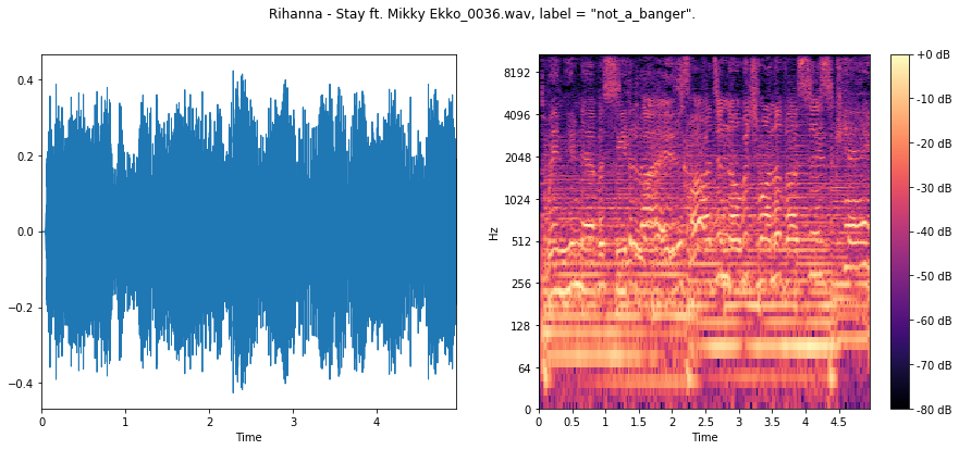
[plot_waveforms(bangerz, i) for i in [0, 1, 2]];
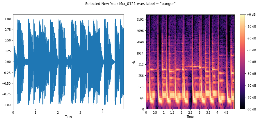
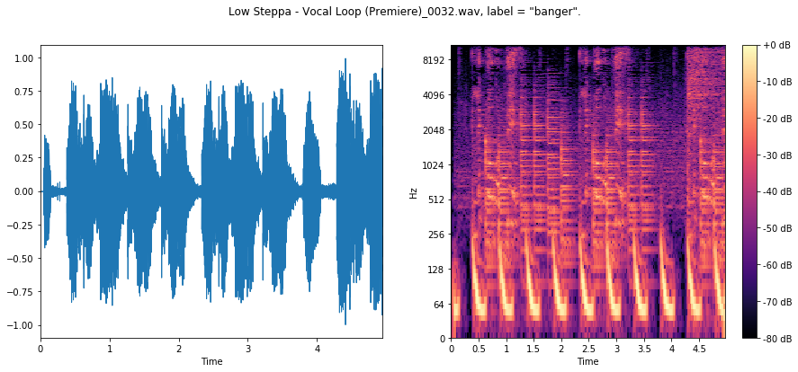
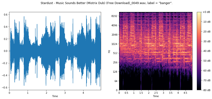
We can see for the first two bangers sharp, rhythmic, percussive signal, focused on the low end of the frequency spectrum. This is the kick drum!
In the third banger, we are likely in a section where the producer has used a high-pass filter, since there is virtually no low-frequency content here, yet we can still see some regularity from the kick in the higher end of the spectrum.
Now for the clangers!
[plot_waveforms(clangerz, i) for i in [0, 1, 2]];
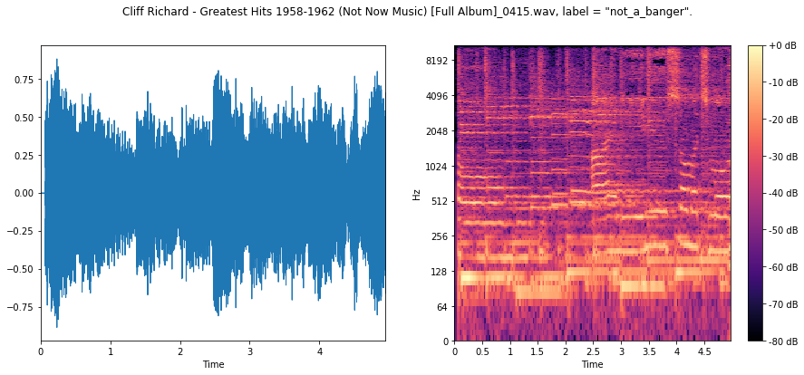
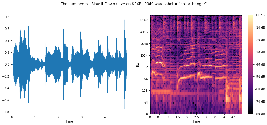
Here we see a less percussive, rhythic signal across the board, with far less low-frequency content.
Hopefully our ConvNet will be able to use this to its advantage.
Establish baseline
We can calculate a baseline classification accuracy, if we just choose the majority label in the dataset for any example. This is the accuracy we need to beat.
Ideally, we should run “Haverford’s algorithm” and compare, but I really didn’t feel like doing this for 875 examples! Volunteers welcome…
    naive_accuracy = (max(num_bangerz, num_clangerz) / (float)(df.index.size))
    print ("This is the accuracy if we always guess max{#banger, #not_a_banger}: %.3f" % naive_accuracy)
This is the accuracy if we always guess max{#banger, #not_a_banger}: 0.518
Form the training and testing data sets
Let’s set aside 80% of the data for training and 20% for testing.
    train_frac = 0.8

    def split_train_test(df, train_frac=0.8):
        include = np.random.rand(*df.index.shape)
        is_train = include < train_frac
        train_data = df[is_train]
        test_data = df[~is_train]
        return train_data, test_data

    train_data, test_data = split_train_test(df, train_frac)


    print( "Training data has %g clips, test data has %g clips." % (train_data.index.size, test_data.index.size))
Training data has 711 clips, test data has 164 clips.
Tensorflow
Having prepped the training and test datasets, we’re ready to set up our ConvNet. We will closely follow the structure of the tensorflow deep MNIST example neural net with some small modifications – if it ain’t broke, don’t fix it!
The deep network will look something like this:
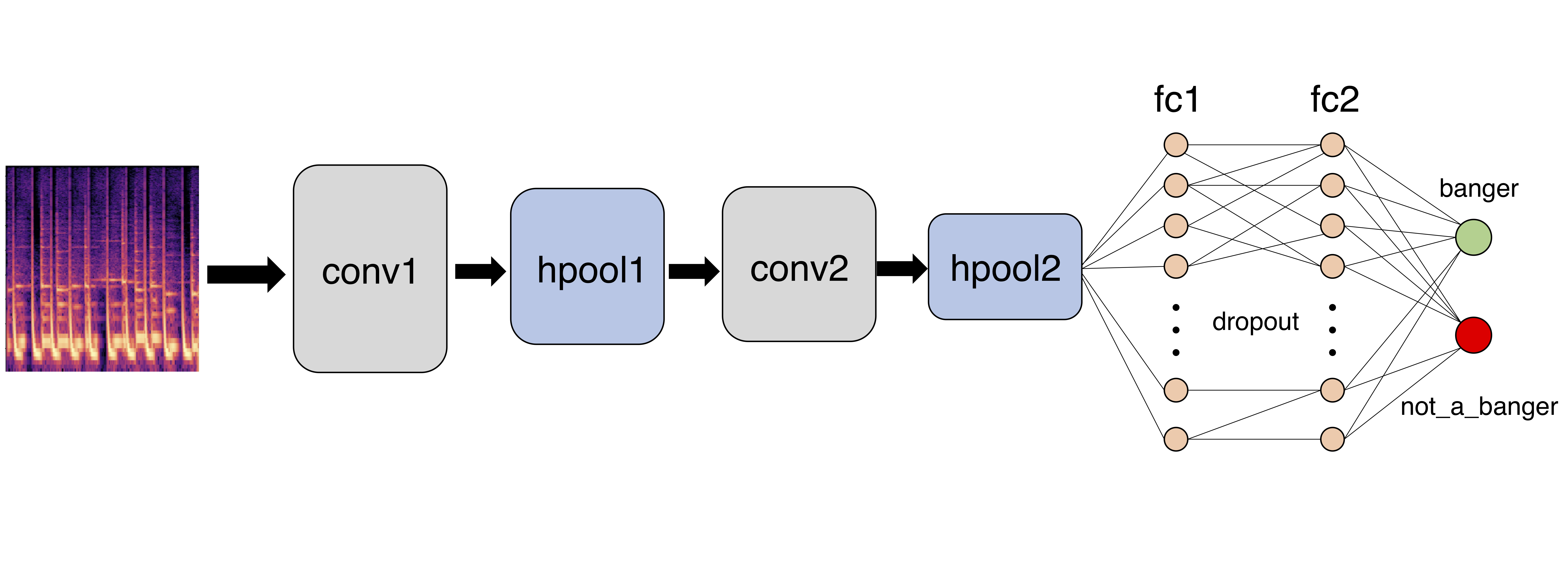
We feed the image of the log spectrogram into a convolutional layer, conv1, followed by a max-pooling layer, hpool1, which reduces the size of the image. We then feed this image into another convolutional layer, conv2, followed by another max-pooling layer, hpool2, which reduces the image size further. We then have two consecutive fully connected layers, fc1 and fc2, between which we use dropout (this randomly removes edges during each epoch of training to mitigate overfitting). Finally, we classify.
We’re going to use the ADAM adaptive moment optimizer, with a cross-entropy cost function.
Setup
    import tensorflow as tf
    tf.set_random_seed(1234)


    # convolution params
    log_specgram_shape = df.iloc[0]["log_specgram"].shape
    CONV_STRIDE_LENGTH = 1
    CONV_WINDOW_LENGTH = 5
    MAX_POOL_STRIDE_LENGTH = 2

    # features
    CONV_1_NUM_FEATURES = 32
    CONV_2_NUM_FEATURES = 16
    DENSE_NUM_FEATURES = 256

    # training
    NUM_LABELS = df.label.unique().size
    BATCH_SIZE = 50
    NUM_EPOCHS = 1000
    LEARNING_RATE = 1e-4
    LOG_TRAIN_STEPS = 1
Draw the computational graph
    # This node is where we feed a batch of the training data and labels at each training step
    x = tf.placeholder(tf.float32,shape=(None, *log_specgram_shape, 1))
    y_ = tf.placeholder(tf.float32, shape=(None, len(df.label.unique())))


    # Weight initialisation functions

    # small noise for symmetry breaking and non-zero gradients
    def weight_variable(shape):
        initial = tf.truncated_normal(shape, stddev=0.1)
        return tf.Variable(initial)

    # ReLU neurons - initialise with small positive bias to stop 'dead' neurons
    def bias_variable(shape):
        initial = tf.constant(0.1, shape=shape)
        return tf.Variable(initial)


    def conv2d(x, W):
        return tf.nn.conv2d(x, W, strides=[1, CONV_STRIDE_LENGTH, CONV_STRIDE_LENGTH, 1], padding='SAME')

    # ksize is filter size
    def max_pool_2x2(x):
        return tf.nn.max_pool(x, ksize=[1, MAX_POOL_STRIDE_LENGTH, MAX_POOL_STRIDE_LENGTH, 1],
                            strides=[1, MAX_POOL_STRIDE_LENGTH, MAX_POOL_STRIDE_LENGTH, 1], padding='SAME')
First Convolutional Layer
We can now implement our first layer. It will consist of convolution, followed by max pooling. The convolution will compute CONV_1_NUM_FEATURES features for each CONV_WINDOW_LENGTH $\times$ CONV_WINDOW_LENGTH patch. Its weight tensor will have a shape of [CONV_WINDOW_LENGTH, CONV_WINDOW_LENGTH, 1, CONV_1_NUM_FEATURES]. The first two dimensions are the patch size, the next is the number of input channels (mono audio, so 1), and the last is the number of output channels. We will also have a bias vector with a component for each output channel.
    W_conv1 = weight_variable([CONV_WINDOW_LENGTH, CONV_WINDOW_LENGTH, 1, CONV_1_NUM_FEATURES])
    b_conv1 = bias_variable([CONV_1_NUM_FEATURES])


    h_conv1 = tf.nn.relu(conv2d(x, W_conv1) + b_conv1)
    h_pool1 = max_pool_2x2(h_conv1)
Second Convolutional Layer
    W_conv2 = weight_variable([CONV_WINDOW_LENGTH, CONV_WINDOW_LENGTH, CONV_1_NUM_FEATURES, CONV_2_NUM_FEATURES])
    b_conv2 = bias_variable([CONV_2_NUM_FEATURES])

    h_conv2 = tf.nn.relu(conv2d(h_pool1, W_conv2) + b_conv2)
    h_pool2 = max_pool_2x2(h_conv2)

    # 2x2 maxpool gives image dimensions np.ceil(np.array(log_specgram_shape)/2).astype(int)
Densely Connected Layer
Now that the image size has been reduced, we add a fully-connected layer with 256 neurons. We reshape the tensor from the pooling layer into a batch of vectors, multiply by a weight matrix, add a bias, and apply a ReLU activation function.
    def scale_shape_maxpool2x2(shape_tuple):
        return np.ceil(np.array(shape_tuple)/2).astype(int)

    log_specgram_shape_reduced = scale_shape_maxpool2x2(scale_shape_maxpool2x2(log_specgram_shape))

    W_fc1 = weight_variable([np.prod(log_specgram_shape_reduced) * CONV_2_NUM_FEATURES, DENSE_NUM_FEATURES])
    b_fc1 = bias_variable([DENSE_NUM_FEATURES])

    h_pool2_flat = tf.reshape(h_pool2, [-1, np.prod(log_specgram_shape_reduced) * CONV_2_NUM_FEATURES])
    h_fc1 = tf.nn.relu(tf.matmul(h_pool2_flat, W_fc1) + b_fc1)
Dropout
To reduce overfitting, we will apply dropout before the readout layer. We create a placeholder for the probability that a neuron’s output is kept during dropout. This allows us to turn dropout on during training, and turn it off during testing.
    keep_prob = tf.placeholder(tf.float32)
    h_fc1_drop = tf.nn.dropout(h_fc1, keep_prob)
Readout Layer
    W_fc2 = weight_variable([DENSE_NUM_FEATURES, NUM_LABELS])
    b_fc2 = bias_variable([NUM_LABELS])

    y_conv = tf.matmul(h_fc1_drop, W_fc2) + b_fc2
Training
Batching function
We need a function to feed in batches of data for training.
    def return_batch(df, batch_size=10):
        batch_df = df.sample(batch_size)
        x = np.vstack(batch_df["log_specgram"]).reshape(batch_df.index.size, *log_specgram_shape, 1).astype(np.float32)
        y = np.vstack(batch_df["label_one_hot"]).astype(np.float32)
        return x, y
Time logging
We want some rough idea of how long training is going to take. On my laptop it was around 14 hours! 😱
    import time

    def estimate_time_remaining(time_in, current_step, steps_gap, total_steps):
        current_time = time.time() - time_in
        time_per_step = current_time / steps_gap
        time_remaining = (total_steps - current_step) * time_per_step
        m, s = divmod(time_remaining, 60)
        h, m = divmod(m, 60)
        print("Approximately %d hours, %02d minutes, %02d seconds remaining." % (h, m, s))
Train and Evaluate the Model
We’re using the numerically stable tf.nn.softmax_cross_entropy_with_logits function here. This is the long part.
    cross_entropy = tf.reduce_mean(
        tf.nn.softmax_cross_entropy_with_logits(labels=y_, logits=y_conv))
    train_step = tf.train.AdamOptimizer(LEARNING_RATE).minimize(cross_entropy)
    correct_prediction = tf.equal(tf.argmax(y_conv, 1), tf.argmax(y_, 1))
    accuracy = tf.reduce_mean(tf.cast(correct_prediction, tf.float32))

    sess = tf.Session()
    sess.run(tf.global_variables_initializer())

    with sess.as_default():
        current_time = time.time()
        for i in range(NUM_EPOCHS):
            batch = return_batch(train_data, BATCH_SIZE)

            # logging
            if i % LOG_TRAIN_STEPS == 0:
                train_accuracy = accuracy.eval(feed_dict={x: batch[0], y_: batch[1], keep_prob: 1.0})
                print('Epoch %d, training accuracy %.3f' % (i, train_accuracy))
                estimate_time_remaining(current_time, i, LOG_TRAIN_STEPS, NUM_EPOCHS)
                current_time = time.time()

            train_step.run(feed_dict={x: batch[0], y_: batch[1], keep_prob: 0.5})
Note: I’ve deleted the output of the above cell to keep the notebook short.
Save model and variables
    with sess.as_default():
        saver = tf.train.Saver()
        save_path = saver.save(sess, "../data/model.ckpt")
        print("Model saved in file: %s" % save_path)

    Model saved in file: ../data/model.ckpt
Testing
Now we have a trained model, we want to test out how well it works on the test set.
    with sess.as_default():
        test_batch = return_batch(test_data, test_data.index.size)
        test_accuracy = accuracy.eval(feed_dict={x: test_batch[0], y_: test_batch[1], keep_prob: 1.0})
        print("Test accuracy: %.3f" % test_accuracy)

    Test accuracy: 0.915
Yay! We have done a lot better than the baseline of 0.518.

What’s Next?
It looks like our initial attempt with a ConvNet trained on log spectrogram data has worked well as a first attempt. However, there are a bunch of things we could think about to improve things:
-
Feature selection: the
librosalibrary which generated the log spectrogram can compute a whole host of different audio features such as mel spectrogram and decompositions of the signal into percussive and melodic components. -
Inspecting misclassified data: digging in to which audio clips were misclassified might give us insight into why they were misclassified. We could use this information to improve the model.
-
ConvNet: There are plenty of hyperparameters to tune here and even the architecture can be changed. Thinking more carefully about the structure of the input features and what design to use could help here.
-
Other models: perhaps another machine learning model, such as SVM or nearest neighbours classification could be more effective (and certainly would be quicker!)
Thanks for reading, and as Tommy H would say, keep it 💯.